File formats
Input
The input contact map is stored as a hash structure using pair-bins as keys. Then, a query is binned into a corresponding key based on its position. The size of the bin is specified by a user (-in_hic_resol for .hic) or dependents on the input file (bin-contact pair files).
HiC map
a bin-contact pair format
-in_bin
A bin file defines the chromosome, start and end positions of each bin, an example: fly_30k.cbins (D.mel in 30k bin).
cbin   chr from.coord  to.coord
 1     2L  6000        7000
 2     2L  7000        8000
 3     2L  8000        9000
 4     2L  9000        10000
 5     2L  12000       13000
-in_map
A contact map contains Hi-C frequency indexed by bins in text format, an example fly_30k.n_contact.
cbin1   cbin2   expected_count  observed_count
 1   1   0.077080    50
 1   2   0.389912    314
 1   3   0.493750    163
 1   4   0.560505    169
 1   5   0.368884    79
expected_count : the expected contact between those two genome locis (bins) according to model. It could be 1 if no model is applied.
observed_count : the observed contact between those two genome locis (bins) in Hi-C data
It takes time to parse text format so we develop bin/genBinMap to turn text format (.n_contact) into binary format (.binmap) which could be used in -in_map, an example fly_30k.binmap.
genBinMap [options] -in_ncontact input.n_contact -out_binmap out.binmap
>bin/genBinMap -in_ncontact examples/fly_30k.n_contact -out_binmap examples/fly_30k.binmap
>hicmaptools -in_map examples/fly_30k.binmap -in_bin examples/fly_30k.cbins -bait examples/bait.bed -output baitTest.tsv
.hic format
The . hic format is generated by Juicer. The parser of . hic is adapted from straw.
-in_hic
A .hic file by applying Juicer on HiC fastq of Galaxy training.
-in_hic_norm (optional)
To extract data based on a specified normalization method, NONE, VC, VC_SQRT, or KR (default: NONE).
-in_hic_resol (optional)
To extract data at a specified resolution, e.g., 5000, 10000, or 50000 (default: 10000).
Query file
The query file is in bed format, where the first three columns are enough. Next, the example of each query mode is listed. Although the biology scenarios of examples are mainly based on Drosophila, HiCmapTools could handle other species (i.e., the example of the mouse Tox gene in the bait query model).
bait: bait.bed a PRE binding site, Tox_mm10.bed mouse Tox gene
local: local.bed a PcG TAD
loop: loop.bed gene, Antp
pair: pair.bed a pair of insulator binding sites
sites: sites.bed a list of insulator binding sites in range 3L:10000000-11000000
submap: submap.bed a region contains Antp-BX long range conttact
TAD: TAD.bed selected TADs in range 2L:2000000~3000000
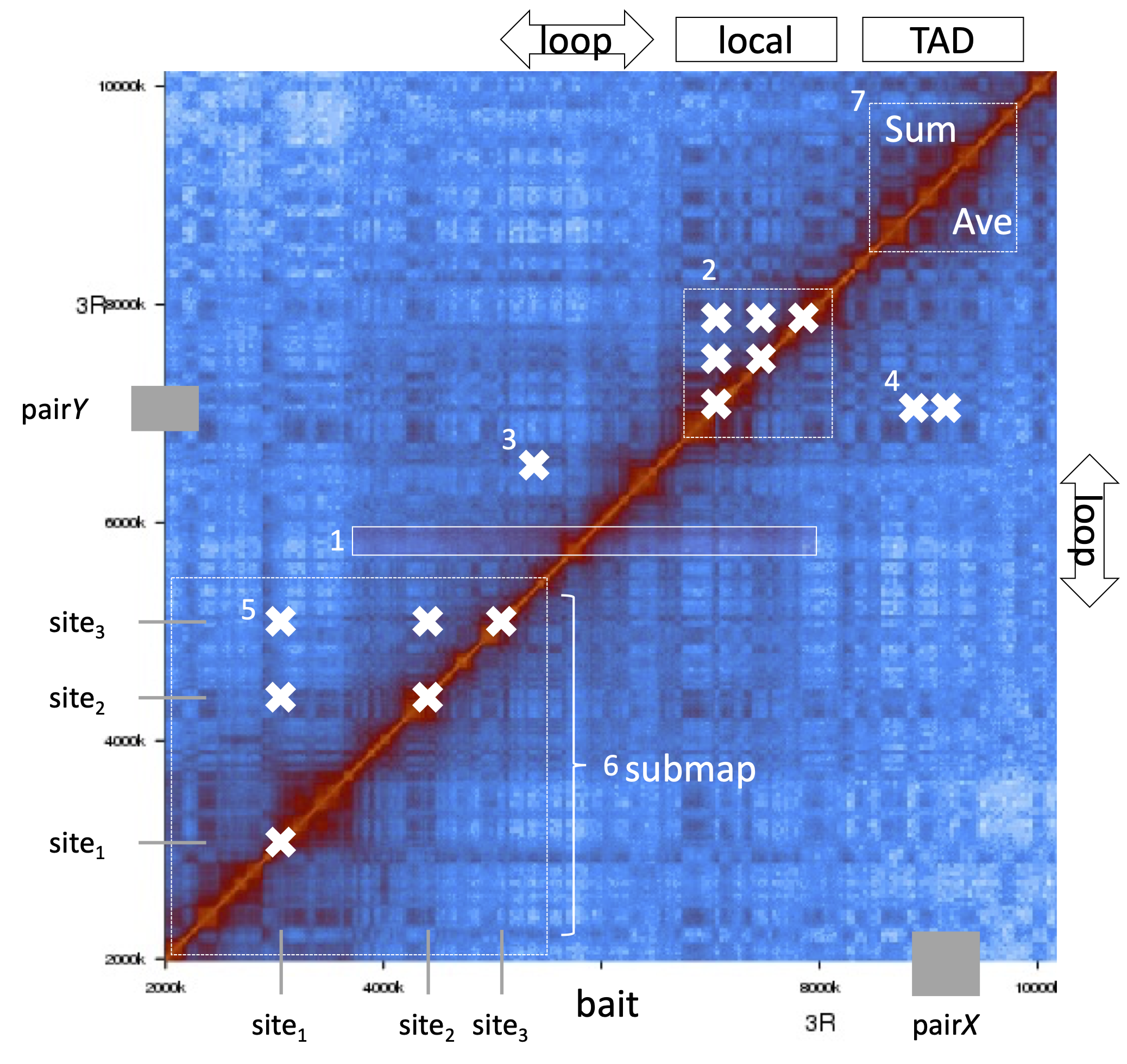
Illustration of query modes
Output
There are two output files. You can use the tool tools/visualPermutationTest.R to examine query’s contact frequency aganist the null hypothesis (Shuffle test).
output.tsv : the contact frequency of the interested regions
sum_* indicates frequency of HiC
rand_* indicates frequency of shuffle test
divide_* indicates ratio of sum/rand
rank_* indicates the rank of HiC among shuffle test. The smaller rank is, the stronger query frequency is (i.e., rank_nor 0.600 = top60%).
index  chrom   start   end     sum_obs sum_exp sum_nor rand_obs        rand_exp        rand_nor        divide_obs      divide_exp      divide_nor      rank_obs        rank_exp        rank_nor
1      2L      594629  595145  47916.000       459.715 2380.531        32618.180       314.679 2525.479        1.469   1.461   0.943   0.100   0.140   0.600
output _random .txt : the observed, expected and normalizated contact intensities of the null hypothesis starting from the third row where the second row is the query frequency
random_obs,random_exp,random_nor
47916,459.715,2380.53
19632,158.539,2956.25
57574,448.25,2832.44
7074,60.7897,3029.22
33009,246.588,3311.8